Example Tutorial

A bundled version of the URC Assessment Method tool can be downloaded from EDX.

For this tutorial, we will be simulating a portion of the Powder River Basin Case Study as outlined in [Creason et al., 2023]. To do this, we will first need to download the publication’s supplementary data from its EDX submission page. Specifically, you will want to download and unzip the file esm_3.zip; you will also need to unzip the file esm_3/PRB- URC Asessment data/DA & DS databases/DA & DS vector database.zip

Initial Setup

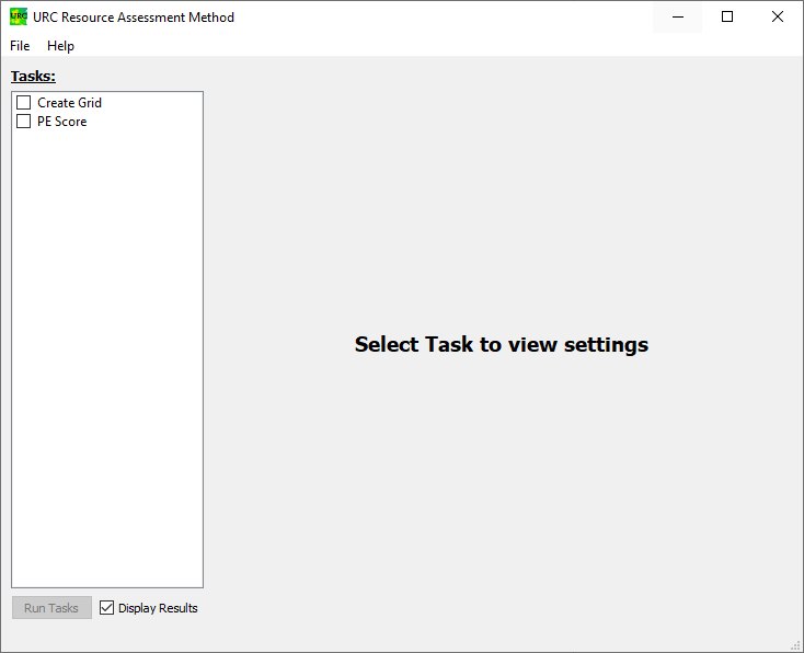
Launch the URC Assessment Method tool:

• If using the Bundled version of the tool, double-click on URC_Assessment_Method.exe.

• If running from source, run urc_assessment_method.py with no arguments.

Once the tool is loaded, you should see a window similar to the image above.

Leave the Display Results box checked.

Configuring the Create Grid Task

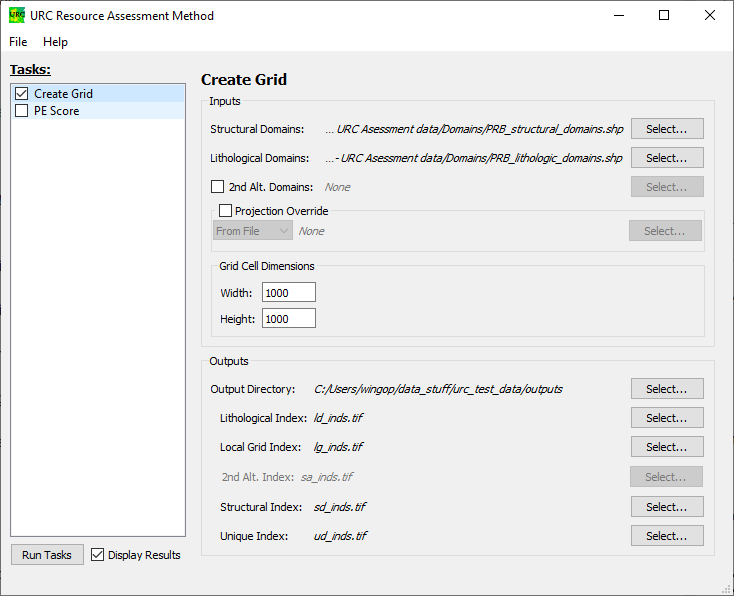
Check the box next to Create Grid; a series of options should appear on the right side.

We will set two of the fields in the Inputs box to some of the files provided in esm.zip. These files are vector map layers containing domains generated by a knowledge expert using the Subsurface Trend Analysis (STA) method, as described by [Rose et al., 2020], and will be used as the foundation for creating the raster-based index grids used for the PE Score Task.

Add the Structural and Lithologic Domains as to the Inputs box:

• Click on the Select… button to the right of the Structural Domains field. Choose the file esm_3/PRB- URC Asessment data/Domains/PRB_structural_domains.shp and click on the Open button.

• Click on the Select… button to the right of the Lithological Domains field. Choose the file esm_3/PRB- URC Asessment data/Domains/PRB_lithologic_domains.shp and click on the Open button.

The Grid Cell Dimensions box describes the width and height of each pixel cell in real-world units. The units are defined by the applied projection; either the current projection of the Structural Domains data source, or the projection provided in the Projection Override box. In this example, the width and height are both in meters.

Feel free to leave the fields in the Grid Cell Dimensions box (both 1 kilometer). If, however you find that the task execution is taking too long to run, you can cancel and increase the grid dimension; a 10 kilometer width and height will significantly reduce the runtime.

The Outputs box allows us to determine where we’d like to save our indexing rasters. We can either give each output its own fully qualified file path, or provide a single directory and relative file names. In this case, we’ll be doing the latter:

• Click on the Select… to the right of the Output Directory. Choose a directory to store the generated index (*.tif) files, and click on Select Folder.

Leave the rest of the fields set to their defaults.

Configuring the PE Score Task

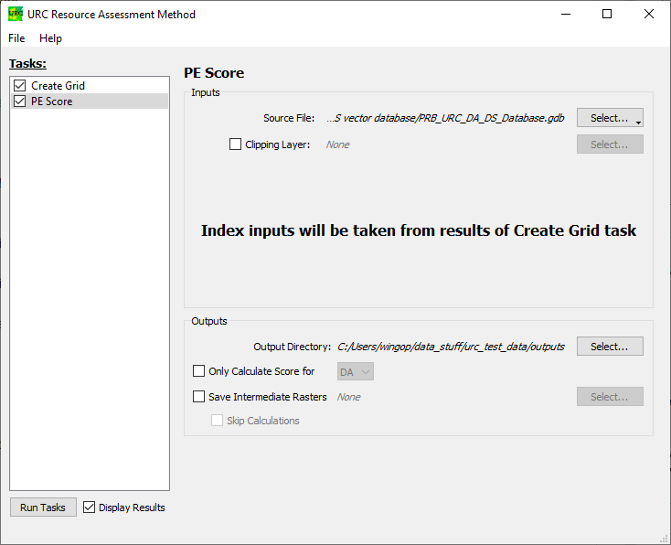
Check the box next to PE Score; once again, a series of options should appear on the right side.

Since we are running both tasks at the same time, there is only one required input for this task: an archive of geospatial data identified according to the guidelines provided in the appendices of [Creason et al., 2023]. This data can come in the form of a FileGeoDatabase (*.gdb) or a Spatialite (*.sqlite) file. If the Create Grid Task were omitted, the Inputs box would require the raster index files that were generated with a previous run of the Create Grid Task.

In the Inputs box, select the data for the Powder River Basin:

• To the right of the Source File label, click on the Select… button, and choose the .gdb file option in the menu. Navigate to esm_3/PRB- URC Asessment data/DA & DS databases/DA & DS vector database/DA & DS vector database/PRB_URC_DA_DS_Database.gdb and click Select Folder.

For the Outputs box, only the Output Directory needs to be set; this can be the same directory as chosen for the Create Grid Task:

• Click on the Select… to the right of the Output Directory. Choose a directory to store the generated scoring files, and click on Select Folder.

The remaining settings in the Outputs box are useful for troubleshooting intermediate steps, or only running one of sets of scores, but are not relevant to this example.

Executing the Tasks

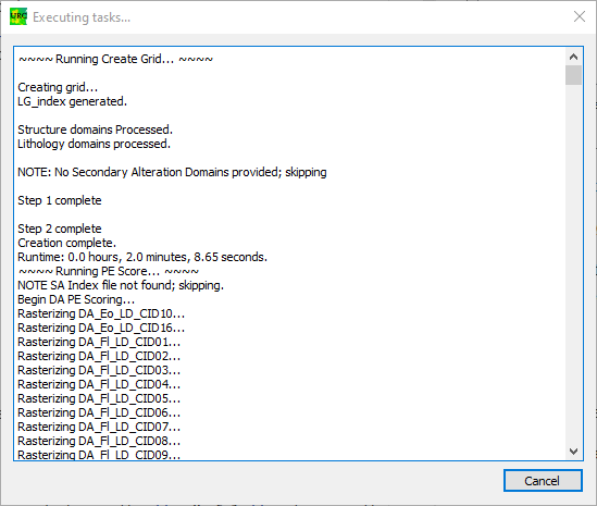
At the bottom of the main window, click on the Run Tasks button. A new dialog should popup and proceed to display log messages.

The Create Grid task should finish quickly; the PE Score task may take up to a few hours to complete.

Previewing the Results

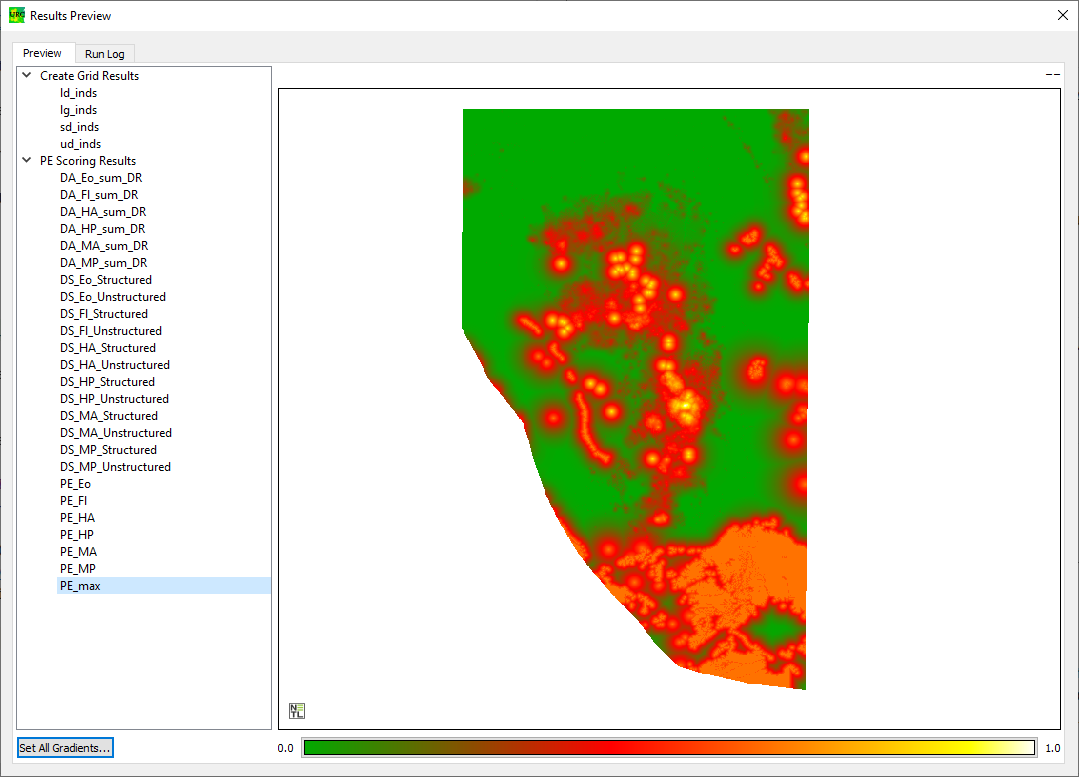
The Raster Geotiff (*.tif) files are intended to be further evaluated in GIS software suites such as ESRI’s ArcGIS or the free and Open Source QGIS. However, the results can optionally be previewed once the tasks completed if the Display Results check box in the main window remains checked.

The output files that were created are sorted by task in a list on the left side of the result dialog. Select PE_max; this will bring up a black and white display of the output file, PE_max.tif. To change the coloring, click on the gradient at the bottom of the dialog. This will bring up a gradient editor.

To the right of the table row with the Start Anchor value, click on the Select… dropdown menu and select Add Below; do this twice. Set the Color and Position values to match the image above (or whatever color values you prefer). Click OK. This will update the color applied to the values for PE_max as displayed in the Results Preview dialog.

The results come in three different flavors:

• The DA_*_sum_DR files capture the Data Available estimates for each defined component.

• The DS_*_ files capture the Data Supporting estimates for both structure and unstructured components.

• The PE_*_ files capture the Potential Enrichment scores for each of the component types, as well as the highest score for each grid cell.

For more information on how to interpret these results, see [Creason et al., 2023].

This concludes the example tutorial. More information on the controls, widgets, and inputs can be found in the Usage section of this user documentation.